The point of this series of posts is to give you an overview of the popular myths and to help you understand what is going on in your Finite-Volume CFD code and how to interpret mesh quality checks for your problem. The goal of this post is to de-mistify the impact of the boundary layer mesh on accuracy.
In the previous post about cell types, it has often been shown that cell types with face pairs are preferred due to the error cancellation effect resulting in significantly lower discretisation error for the same number of cells. This post aims to discuss how this applies to the boundary layer and why is important to resolve boundary layers accurately. The analysis will be presented using some examples of the laminar and turbulent boundary layer and discuss how the mesh influences the accuracy of the simulation. Some mesh guidelines will also be given. It is always beneficial to follow our Tips and tricks for generating high-quality meshes, too.
The laminar flow between two parallel plates
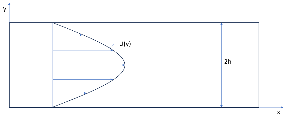
This type of flow has an analytical solution and therefore serves as a good example. Please note that the convection term vanishes in this case, and only the Laplacian (diffusion) term is relevant. The velocity profile can be written:
Where μ is the dynamic viscosity and h is half of the height of a channel.
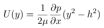
By looking into the derivatives of the solution, it can be found that:
- The first gradient of velocity is:
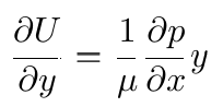
- The second gradient of velocity is:
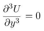
- The third gradient of velocity is:
Some conclusions can be drawn here:
- The flow is one-dimensional, therefore, is beneficial to resolve with cell types having face pairs in the y direction.
- The error in the x direction is always zero irrespective of the type of cell used, because the solution is uniform and can be resolved exactly with any type of mesh.
- This solution does not require a very fine prism layer near the wall and can be resolved accurately using coarse meshes.
Developed turbulent boundary layer
A developed turbulent boundary layer can be considered as a one-dimensional flow where the velocity changes rapidly from the wall to the bulk of the flow.
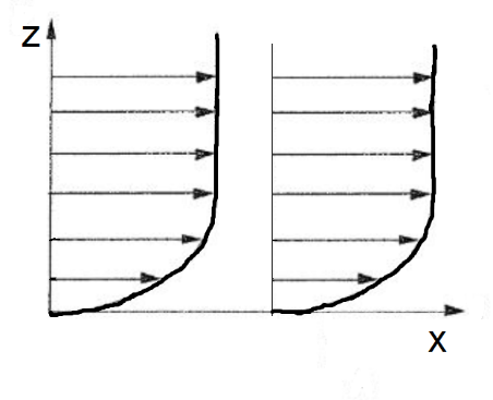
It is well known that a turbulent boundary layer can be divided into three major parts:
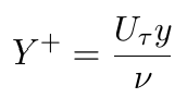
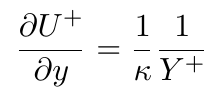
The viscous sub-layer – is a thin part near the wall where the viscosity forces are dominant and the flow is laminar due to the influence of the wall. It stretches from 0 < Y+ < 5 where Y+ is the non-dimensional distance from the wall:
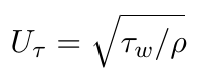
Uτ is the so-called friction velocity:
The buffer layer – is a part of the layer where both viscous and turbulent stresses are comparable. It is part of the layer where 5 < Y+ < 15 -30.
The log-layer – is part of the layer where the turbulent stresses are dominant and the laminar stresses are negligible. It ranges from Y+ > 15 – 30, and extends over the outer parts of the layer, and behaves according to the law of the wall:
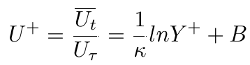
Ut is the friction velocity, κ = 0.41 is a Von Karman constant, and B=5.2 for a layer over a flat plate.
In this situation, a complete set of Reynolds Averaged Navier-Stokes equations, using the Boussinesq Eddy Hypothesis, reduces to a one-dimensional equation:
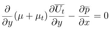
Where the pressure drop in the streamwise direction is in balance with friction forces at the wall, and μt is the so-called turbulent viscosity, calculated using a turbulence model.
Turbulent flows, especially at high Reynolds number, impose the biggest challenge in modeling boundary layers because of rapid velocity variation at the wall. The above equations show that:
- Rapid velocity variation is present in the direction normal to the wall.
- Convection terms vanish in the boundary layer and therefore do not contribute to discretisation errors. Hence, the choice of the interpolation scheme for the convection term does not play any role in the developed boundary layer flows.
- Friction stresses are modeled using the Laplacian term and the turbulent viscosity is calculated by the turbulence model.
Let us now discuss how the physics of the boundary layer influences meshing and provide some guidelines on how to get the best accuracy for a given problem. It was mentioned before that the stress in the boundary layer is governed by the Laplacian term, and in the previous posts we have shown that:
- Cell types with face pairs in the direction normal to the wall are desired for achieving the best possible accuracy. The type and orientation of base faces are not relevant because there is not much variation in the streamwise direction, and this makes any mesh produce exact solutions. Any type of prismatic cell satisfies this condition.
- Non-orthogonality in the direction normal to the wall shall be minimised. Hence, it is important to keep non-orthogonality at base faces low inside the boundary layer, especially at the wall. Non-orthogonality at other faces is not important because the flow is uniform in the streamwise direction.
- The mesh shall be as uniform as possible to improve the prediction of surface-normal gradients over face pairs.
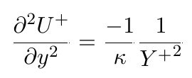
Let us analyse in more detail how mesh uniformity plays a key role in achieving the accurate representation of the boundary layer, and it, therefore, requires more attention. From the log of the wall, it stems that velocity gradients are largest at the wall and they quickly decline as the distance from the wall increases. For example:
- The first gradient of velocity is:
- The second gradient of velocity is:
- The third gradient of velocity is:
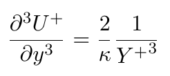
In the previous post about cell types, it was shown that the discretisation error for the Laplacian term is proportional to the third gradient in the direction normal to the wall. Therefore, a cell type with face pairs in the direction normal to the wall is needed. The solution is mostly uniform in the flow direction and therefore any mesh can resolve it accurately. The equation for the third gradient of velocity shows that the gradient reduces to the power of three with the distance from the wall. This means that the discretisation error of the velocity field reduces quickly by moving away from the wall, and any type of mesh with any density can resolve it accurately at a certain distance from the wall. Furthermore, it shows that it is important to focus on getting high-quality layer cells with a small thickness ratio in the inner part of the layer where the gradients are still significant and that thickness ratio can be increased in the outer part of the layer to save on computational resources without sacrificing accuracy. In addition, it also shows that enforcing an extreme total thickness of the layer is not necessary and, therefore, it is not needed to enforce the mesh to cover the total thickness of the layer to achieve the accurate solution. Please also bear in mind that other turbulent quantities, like turbulent kinetic energy, turbulent dissipation, etc. decay quicker than the velocity in the log-layer and the above analysis is also valid for them.
Key takeaways
The most important takeaways about the meshing of boundary layers are:
- Strong gradient variation is present in the direction normal to the wall
- Prismatic elements, with face pairs in the direction normal to the wall, are needed to resolve the layer accurately with the smallest possible error.
- The discretisation error reduces quickly with the distance away from the wall, hence, it is important to focus on having smooth thickness variation in the inner part of the layer, to resolve the shear stress accurately.
I hope that you have found this post useful and that it has made you curious to use the knowledge presented in this post, try out our latest CF-MESH+, designed to alleviate you from the pain of meshing. You can also subscribe to our newsletter to stay informed on our newest developments.
- cfMesh 1.2 Released — Introducing a Full GUI for Streamlined Meshing Workflows
- How to install a trial version of CF-MESH+
- Our best meshing practices for high-quality CFD simulations
- Is it always the mesh? Part 7: Volume Ratio – the Secret Killer Nobody Talks About
- Automatic Acute Edge Detection and Fillet Creation Algorithm
")
