Quite often I hear complaints about non-orthogonality and skewness, and how it’s worthless even trying to run a solver on a mesh, etc. The point of this series of posts is to give you an overview of the popular myths and to help you understand what’s going on in your Finite-Volume CFD code and how to interpret mesh quality checks for your particular problem.
The first question that shall be answered is how are mesh-quality metrics defined. Their influence on mesh quality will be analysed later in the context of terms commonly occurring in partial differential equations.
Let us start by defining the mesh first. By definition, the mesh is a subdivision of the computational domain into so-called cells, used for the approximation of governing laws.
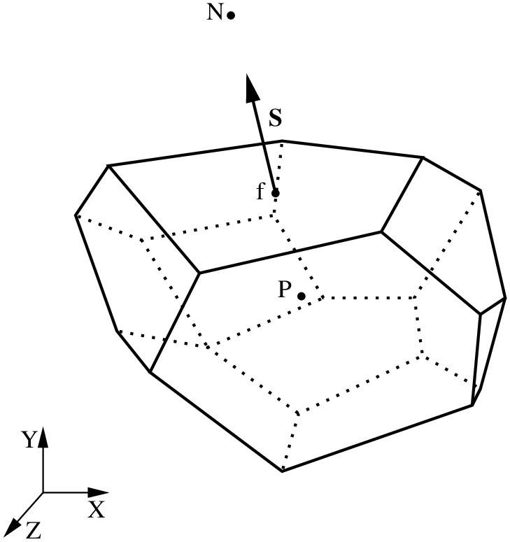
The figure above shows a cell in a mesh, and each cell in the mesh shall satisfy the following properties:
- No overlap – cells may share a common face, edge or vertex. This criterion ensures the conservation of properties under consideration across the domain.
- Cells and faces shall be convex – this ensures that the centroid is inside the cell.
- Consistent orientation of face normal – this is needed to simplify the implementation of the discretisation schemes for the governing laws.
Mesh quality metrics
Non-orthogonality
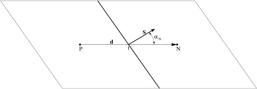
Non-orthogonality is measured as an angle between the surface-area vector and the line connecting the centres of cells adjacent to a face. In a valid mesh, non-orthogonality shall be in the interval between 0 and 90 degrees. Lower values are desired!
Skewness
Skewness is measured as the relative distance between the face centre and the point where the line connecting the neighbouring centres of a face intersects the face and the distance between the neighbouring cell centres. Skewness does not affect the validity of a mesh. However, lower values are desired!
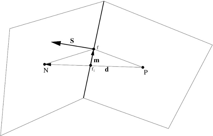
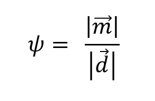
The definition of skewness is:
Face uniformity
Face-uniformity is measured as a ratio of the distance from the face centre to the neighbour cell centre over the distance between the cell centres.
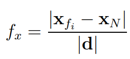
Where xfi and xN are the face centre and the neighbour cell centre, respectively, as shown in the figure above. The ideal value is 0.5. It is beneficial to keep the uniformity as close to 0.5 as possible! Lower values do not make the mesh invalid. However, it has a negative effect on accuracy!
Finite Volume Discretisation
The most common terms, occurring in continuum mechanics, can be classified as temporal, convection, divergence, diffusion and source terms.
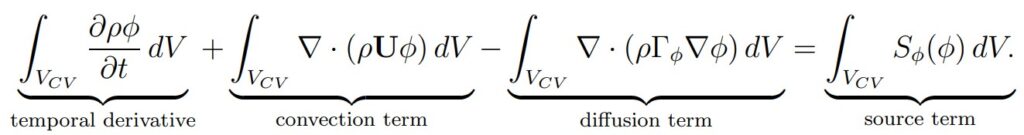
This post is not about the theory of fluid mechanics, Lagrangian, Eulerian approach, etc. Hence, I wish to focus on the discretisation of terms and the corresponding mesh quality metrics associated with each term. Temporal terms do not require a mesh and will not be discussed either. The main focus is on spatial terms because they are affected by the mesh. The discretisation shall satisfy important properties such as:
- Consistency: the approximation error tends to zero with mesh refinement.
- Stability: the schemes shall not magnify numerical errors in the solution process.
- Conservation: numerical schemes shall provably obey conservation laws, both globally and on a cell-by-cell basis.
- Boundedness: Some physical properties lie within certain bounds, such as density, energy, etc. A numerical scheme shall ensure these bounds are satisfied during the solution process.
The important properties of Finite Volume discretisation are:
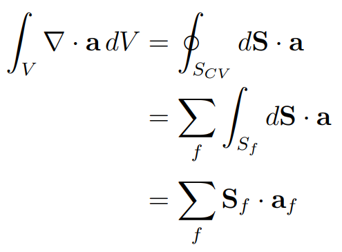
- Conservation laws are integrated over a domain.
- Conservation laws are valid on a cell-by-cell basis.
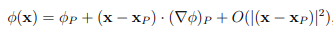
Most often, the values are stored at the cell centres, because a cell centre is a Gauss point:
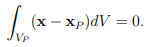
By doing so, it is possible to store only the values at cell centres and still obtain a second-order accuracy. By assuming a constant gradient over a cell, an expansion into a Taylor series can show that the first truncation term is of second order:
Let us now see what happens when the most common terms a discretised.
Source terms
The source term is often linearised to increase the stability of the procedure,
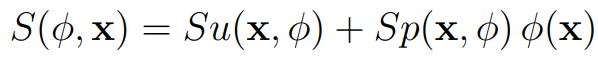
and its integral form is:
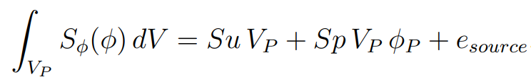
The truncation error of the procedure has the form:
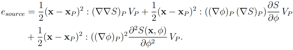
It depends on the size of the cell and the linearisation procedure. The approximation is second-order accurate.
Gradient terms using Gauss type of approximation
The gradient is calculated as a sum of integrals of cell faces:
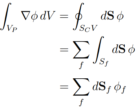
Where Sf represents a face area vector. By using the Taylor series expansion, a truncation error can be found:
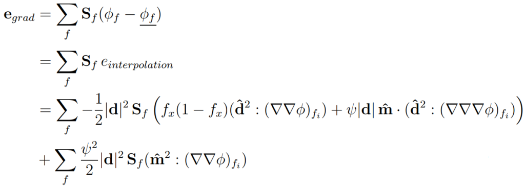
This is interesting because it lets us draw some interesting conclusions that the error depends on:
- Cell size
- The solution itself
- The type of the cell
- Skewness
- Uniformity
Divergence terms
Divergence is calculated as a sum of integrals over cell faces:
The truncation error has the following form:
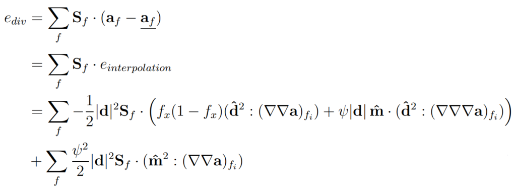
As we have already noticed before, the error depends on:
- Cell size
- The solution itself
- The type of the cell
- Skewness
- Uniformity
Key takeaways
I have presented the most common mesh quality metrics used for assessing the quality of the mesh and briefly presented their influence on the discretisation practice. Please remember a few important takeaways:
- Non-orthogonality, skewness, and uniformity do not affect the accuracy of source terms. The accuracy depends only on the size of the cells and the error tends to zero with mesh refinement. This means that when the source terms behave in an obscure manner, it makes sense to refine the mesh or revise their linearisation practice.
- Non-orthogonality does not affect accuracy on divergence, gradient, and source terms and is not the most important quality metric for convection-dominated flows. It is an important measure in the viscous part of the boundary layer, and we will discuss this topic in one of the future posts.
- Skewness and uniformity affect the accuracy of divergence and gradient terms. It is important to note that this is only the case in regions where the solution is not uniform! In practice, this means that the mesh shall be of high quality in shear layers, and jets, where the solution exhibits rapid variation!
In future posts, I will discuss the convection and Laplacian terms in more detail and discuss the influence of mesh quality on the accuracy of the FV discretisation practice.
I hope that you have found this post useful and that it has made you curious to try out our latest CF-MESH+, designed to alleviate the pain of meshing. You can also subscribe to our newsletter to stay informed on our newest developments.
- cfMesh 1.2 Released — Introducing a Full GUI for Streamlined Meshing Workflows
- How to install a trial version of CF-MESH+
- Our best meshing practices for high-quality CFD simulations
- Is it always the mesh? Part 7: Volume Ratio – the Secret Killer Nobody Talks About
- Automatic Acute Edge Detection and Fillet Creation Algorithm
")
