This case study shows the methodology for the generation of multi-material meshes in heat exchangers. In most cases, the device is designed by many engineers, resulting in imperfect CAD data with overlaps and self-intersections. CF-MESH+ does not require perfect CAD data and offers utilities to clean up overlaps which may sometimes be problematic.
Most solvers require the mesh to be in SI units, which can be easily achieved by our scaling utilities. In a multi-domain simulation, it is often necessary to provide meaningful names to the subdomains in the mesh, and this can be achieved by providing a boundary region unique to a given domain. This simplifies the setup for imperfect CAD data. Various types require different handling of internal interfaces. By default, CF-MESH+ generates a boundary region at the internal interface, and it can easily be converted to ordinary internal faces when needed. A robust procedure for the generation of prismatical cells in the boundary layers offers 100% layer coverage even for complex geometries. In addition, it offers numerous options to specify refinement in regions where small cells are necessary.
Geometry preparation
Simulating a shell and tube heat exchanger can be a very daunting task, due to complex geometry that is difficult to mesh and complex physics requiring a fine mesh in the boundary layer to get accurate heat flux. This task requires a surface mesh to be as clean as possible. The most common problems occurring in geometries are unresolved self-intersections and overlaps. In order to clean these problems, CF-MESH+ offers utilities to Clean surface duplicates and Remove parts that can be used to delete duplicate and unnecessary faces. However, the utility Remove parts should be used with caution, not to remove the parts that shall remain in the geometry. The algorithms in CF-MESH+ are fault-tolerant, as long as the defect is smaller than the required local cell size. This is especially important for multi-domain meshes, where large gaps in the geometry may cause invalid domain definitions.
If you are not confident about how to do it yourself, you can always contact our support. We are aware this process can be automated further, and we plan to release a novel automatic procedure for surface clean-up in the near future. You can subscribe to our newsletter to stay tuned for future updates.
Here you can find more tips and tricks on how to prepare your geometry and provide meaningful settings.
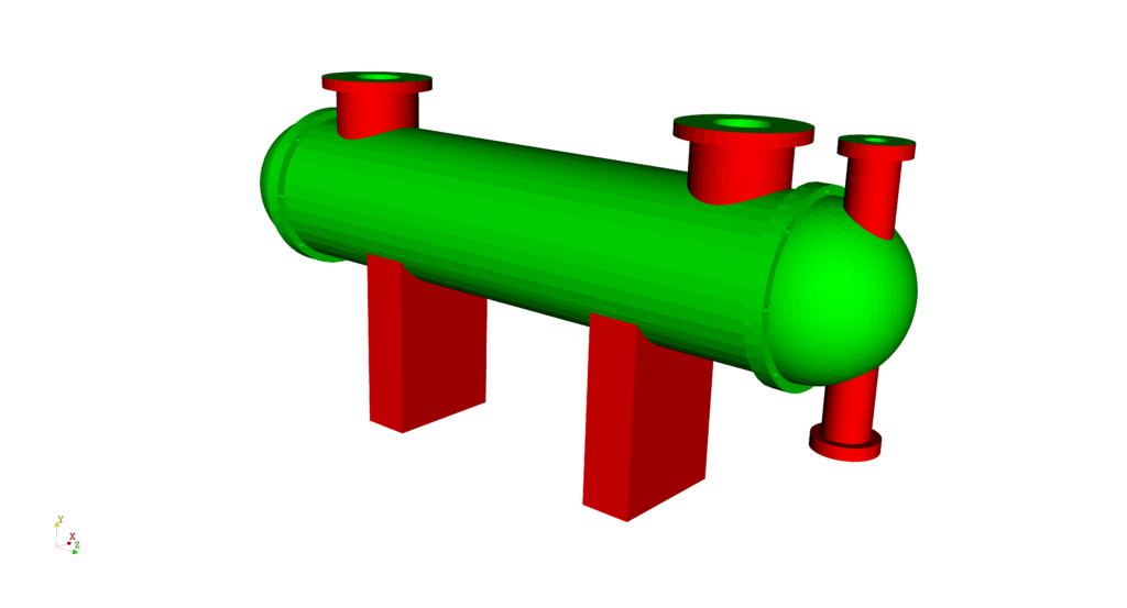
In most cases, the pipes of the heat exchanger can be treated as zero-thickness walls, because the heat flux resistance through the pipes is negligible. The geometry under consideration had a finite thickness wall, and one side of the surface was removed, using the Remove parts utility.
If your engineering judgment tells you that you should model the mesh inside the pipes, as a solid region, please be aware that this requires a lot of cells to mesh the pipes, because the mesher requires at least two cells across the thickness of the pipe, to get a high-quality mesh. In addition, it is a good practice to check the dimensions of the geometry, prior to any changes in the surface mesh. This is not important for the mesher, but for the solver, because most solvers require standard SI units. In our case, the heat exchanger was designed in millimeters so it was scaled by a factor of 0.001, using the Scaling utility, to convert the mesh to metres.
Meshing process
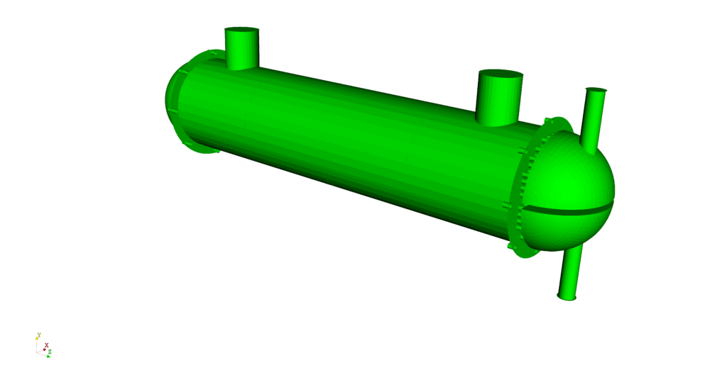
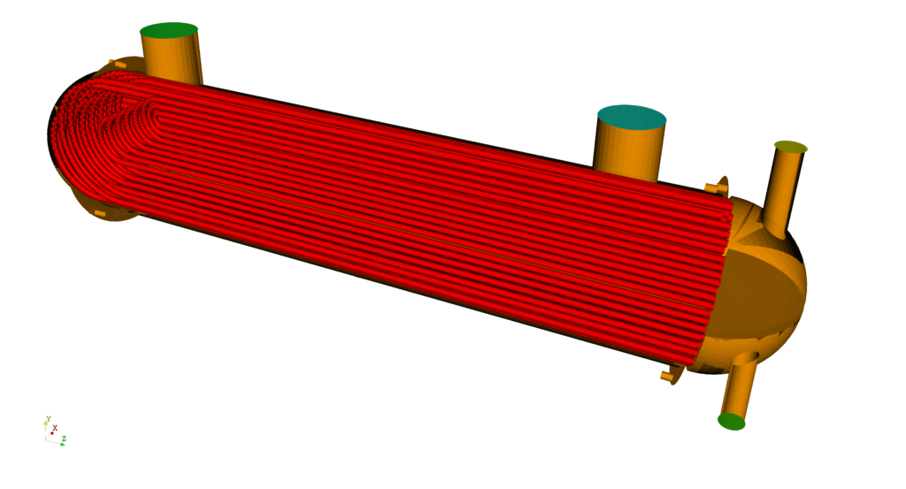
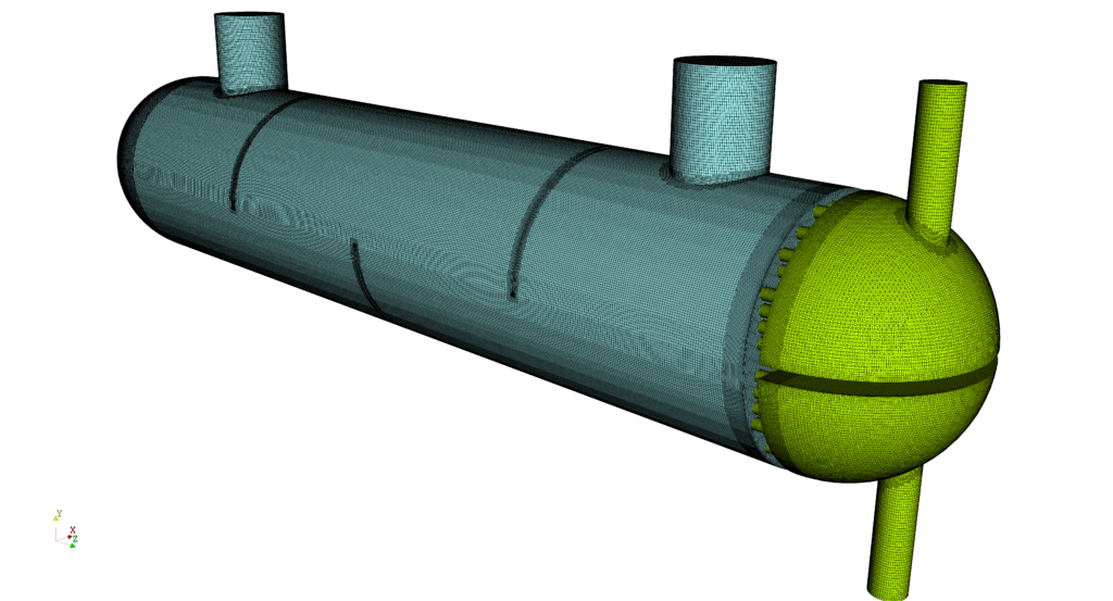
The first step of the meshing process in CF-MESH+ is the definition of patches (boundaries) on the surface mesh. For a closed system, only 2 patches are needed (shell, tubes) to get a valid mesh. However, the heat exchanger is an open system, where both fluid streams have their inlets and outlets. Thus, 6 boundary regions are defined (shell, tubes, inlet, and outlet of fluid 1 and inlet and outlet of fluid 2).
The exchanger is 2.5 meters long. CF-MESH+ has the option to visualize the selected cell size at a given location. By inspecting the geometry, the maximum cell size of 0.01 m was set in the master settings.
In order to get an accurate heat exchange between the fluid streams, the multi-domain capability in CF-MESH+ was used to get a conformal mesh interface between the two streams with high-quality boundary layers. In addition, it is also needed to tell the mesher which parts of the mesh belong to a given fluid. CF-MESH + has a convenient way to define the domains, by using the boundary regions, unique to a given domain. More precisely, the inlet and the outlet of the fluid hot stream, and the inlet and the outlet of the cold fluid stream were used. This way, the two cell zones were generated. Alternatively, it is also possible to define the domains using Point in the domain option. However, this was considered more complex in this case.
By default, CF-MESH+ treats internal interfaces in the mesh as patches where boundary conditions can be specified. However, to run the CHT simulation in OpenFOAM, the interfaces are generated using the splitMeshByRegions utility which does not work well if the interface between the cold and the hot fluid streams is meshed as a patch. In order to generate the mesh without the boundary region at the interface, an option patch conversion to face zones is available in CF-MESH+. It removes faces from the patch tubes and leaves only the ones at the outer boundary of the mesh. A face zone is created consisting of the faces deleted from the patch.
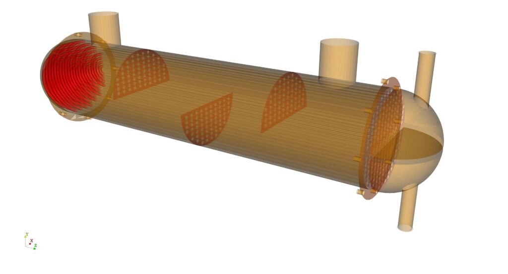
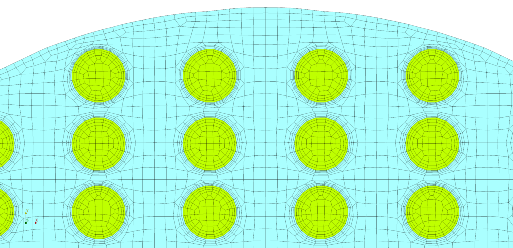
Once the geometry is cleaned and the boundary regions defined, the next step is to choose adequate cell sizes over the domain. A good rule of thumb is to have at least two cells across the gap or radius. For this purpose, CF-MESH+ offers various refinement options, from automatic cell sizing to manual ones. In this case, the regions were defined near the patches shell and tubes and they were used to refine the mesh to get sufficient resolution. In addition, it is recommended to create edge and face subsets and use them to define additional refinement regions, where needed. Such regions are: the pipes’ U-turn, a region where the fluid enters and exits the pipes, internal baffles, etc.
It is recommended to use the Show cell size tool, when choosing the refinement level to compare the selected cell size, with the nearby geometry, such that the optimal cell size can be chosen for the particular region.

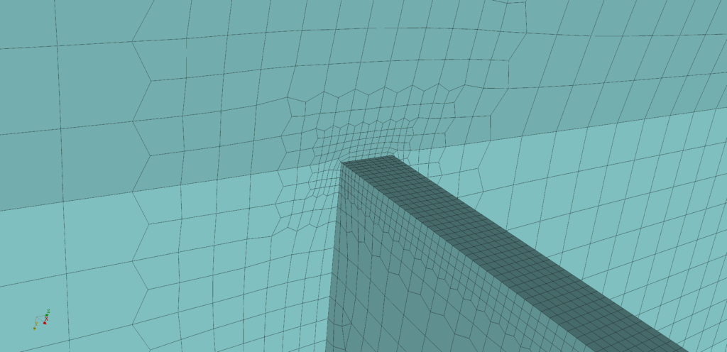
Prismatical cells in the boundary layer are essential for obtaining an accurate heat exchange rate between the two streams. Therefore, it is important to use several layers of prismatical cells on both sides of the tubes. Depending on the goal of the simulation, and the required accuracy of the heat flux, determines whether a low Reynold or a high Reynolds to turbulence modeling is needed. If the low Reynolds modeling is needed, it is necessary to achieve y+ of 1 or smaller, at the pipes wall and this can be achieved by selecting a large number of layers with a small thickness of the first layer.
In this simulation, we decided on a high Reynolds approach, using the wall functions and we selected three boundary layers on both sides. A low Reynolds simulation will come in the future, so make sure to follow our announcements. On other walls, there is no significant heat exchange and they are modeled as adiabatic walls, hence, only 1-2 layers are sufficient there.
Additional meshing steps
By default, the geometry consists of very short outlet pipes where it is not possible to get developed at the outlet. In order to extend the outlet regions for both streams, it is recommended to use the extrudePatch utility. By doing so, it is possible to achieve a uniform flow at the outlet of the domain, resulting in better convergence and a shorter time to get the results.
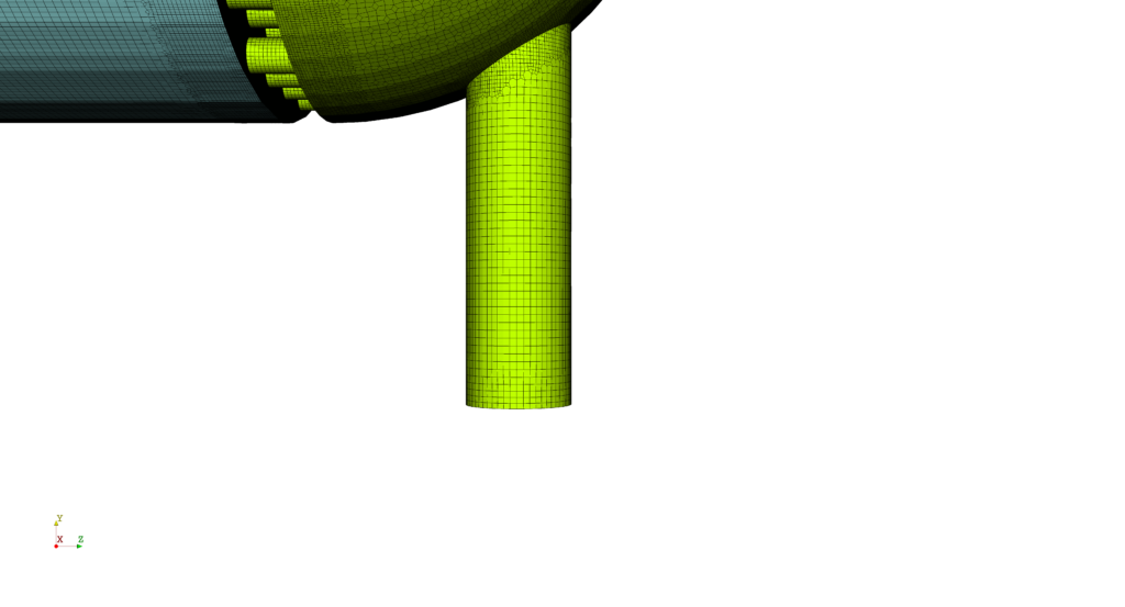
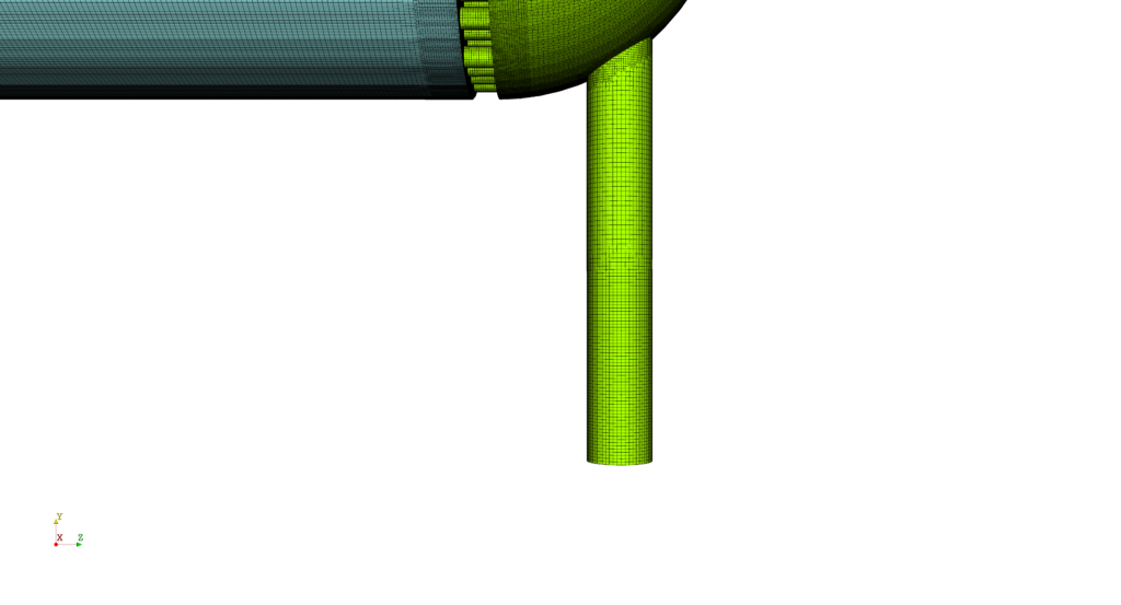
Figure 10: Outlet region after extrusion
Simulation setup
For the heat transfer analysis of this heat exchanger, we used a solver chtMultiRegionSimpleFoam available in OpenFOAM-v2206. A command splitMeshRegions -cellZones -overwrite was used to create two fluid regions, where each one has its own mesh and boundary conditions.

Using low-Reynolds modeling without wall functions
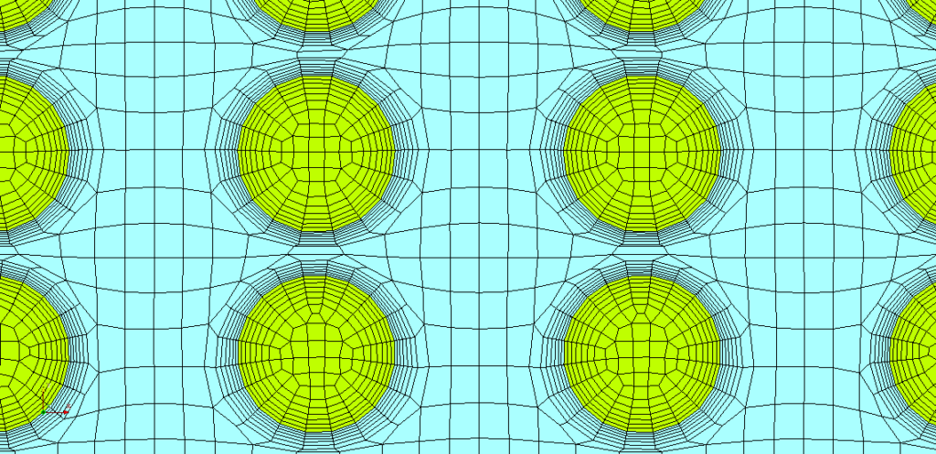
The mesh was constructed using the firstLayerThickness option in boundary layer settings. The setting maxFirstLayerThickness has been removed and does not exist in versions 4.2 and newer. At the pipes boundary, the first layer thickness was defined, according to the predicted velocity, to satisfy the y+ condition. Six layers were applied on both sides of the patch, with an inner thickness ratio of 1.15, the first layer thickness of 0.0005 m, and 3 layers in the outer part of the boundary layer. With these parameters defined, the algorithm calculates the outer thickness ratio to provide a smooth transition to the rest of the mesh. No wall functions were used for the simulation.
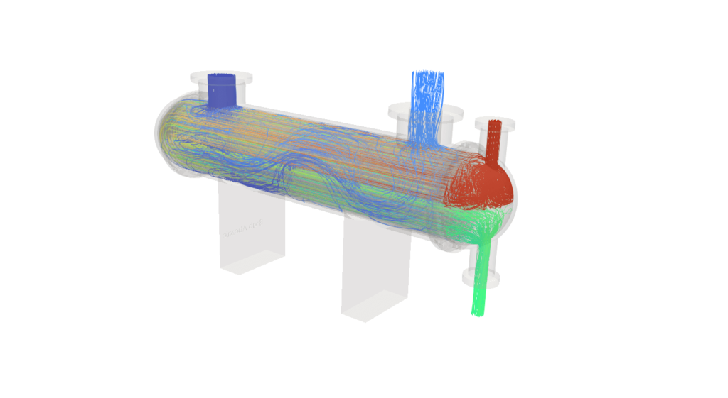
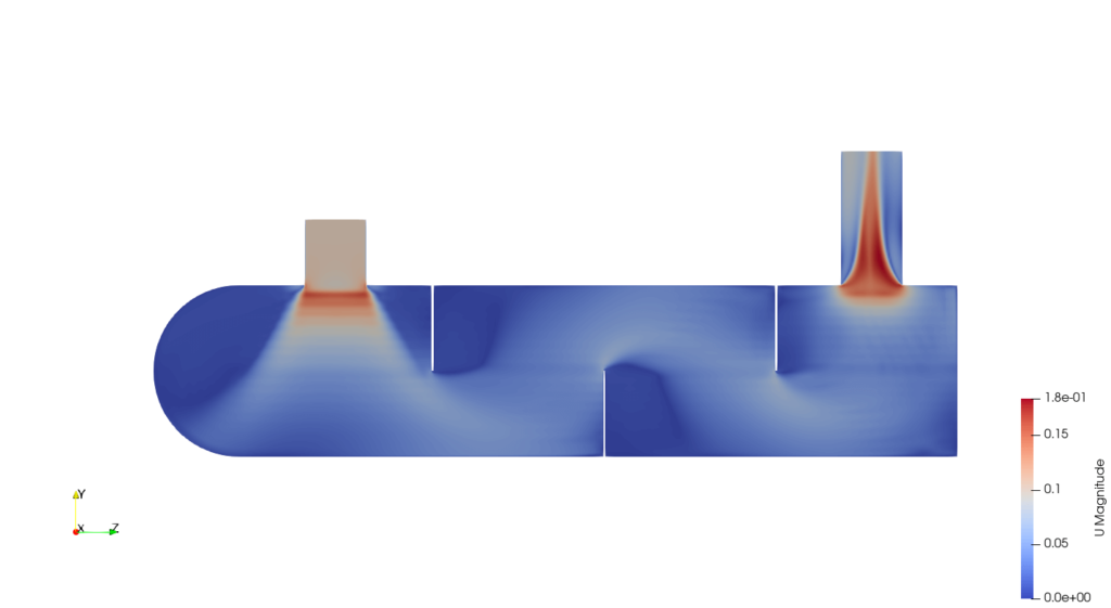
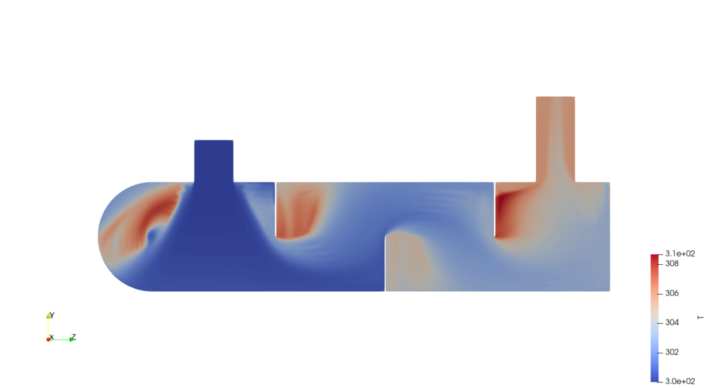
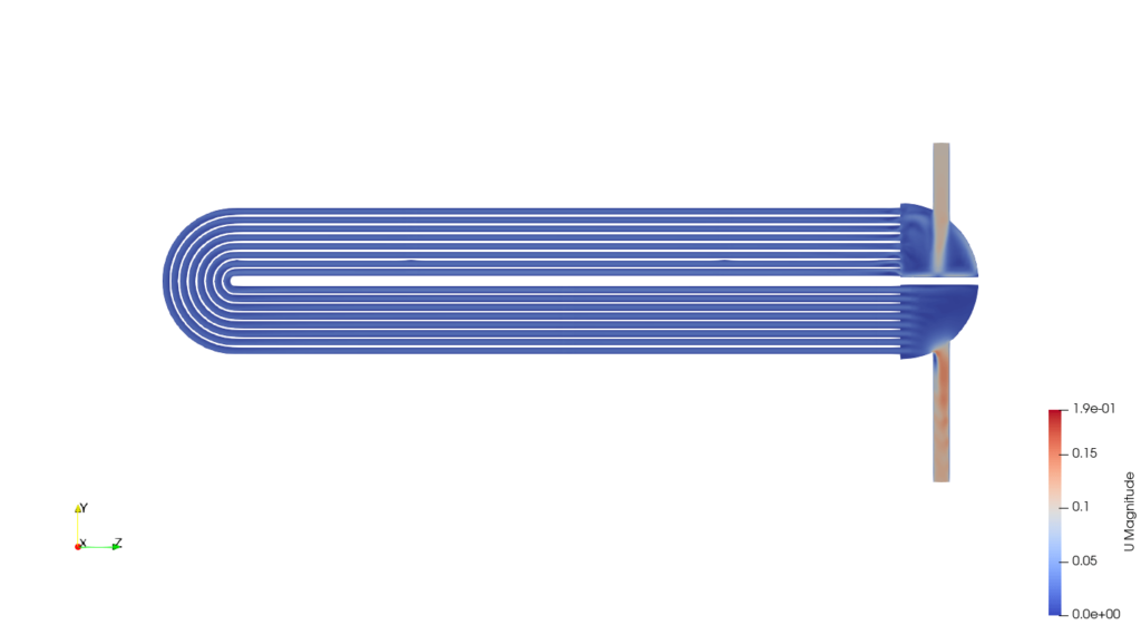
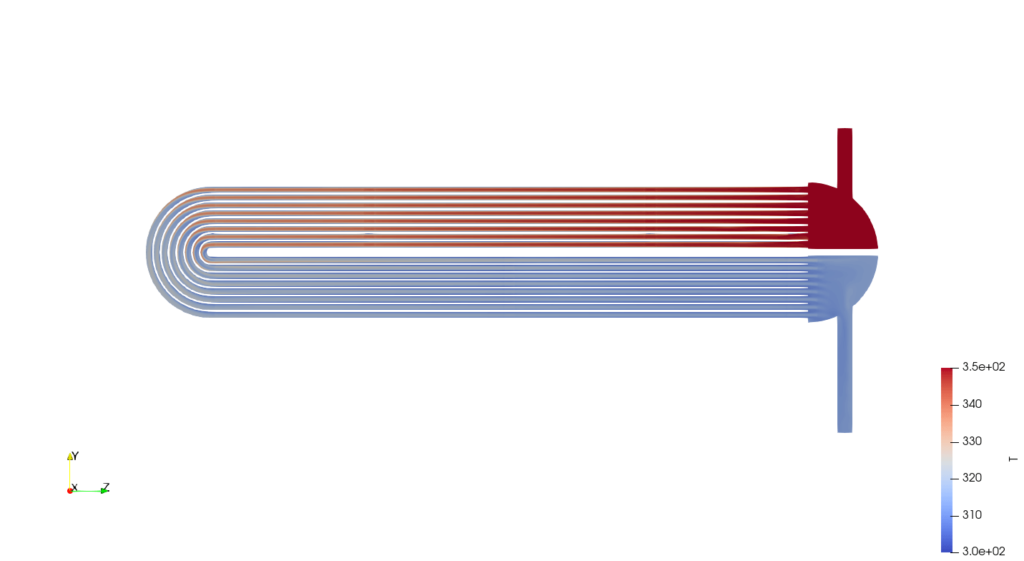
A closer look at the mesh, at the mentioned patch, is given in Figure 13. below. Furthermore, the temperature and velocity distributions, for both fluid 1 and fluid 2, are given in Figures 14 -18. Both fluids enter the domain with velocities of 0.1 m/s, but the temperature of fluid 1 is 350 K at the inlet, where the average temperature of fluid 2 is 300 K. Fluid 1 leaves the domain with an average temperature of 305 K, and fluid 2 with 313 K. Average y+ on the patch pipes on fluid 1 side is 0.43 and on fluid 2 side 0.55.
If you wish to study these simulations in more detail, they are available for download.
We hope that you have found this post useful and that it has made you curious to try out our latest CF-MESH+, designed to alleviate the pain of meshing. You can also subscribe to our newsletter to stay informed on our newest developments.
By Karlo Jurina and Franjo Juretić
- cfMesh 1.2 Released — Introducing a Full GUI for Streamlined Meshing Workflows
- How to install a trial version of CF-MESH+
- Our best meshing practices for high-quality CFD simulations
- Is it always the mesh? Part 7: Volume Ratio – the Secret Killer Nobody Talks About
- Automatic Acute Edge Detection and Fillet Creation Algorithm
")
