The goal of this post is to discuss the best practices of boundary layer generation in CF-MESH+ needed to perform low-Re turbulence modelling of boundary layers, on Ahmed body example. In order to show the importance of accurate boundary layer modelling, the post presents the results obtained on cartesian and tetrahedral meshes with the similar number of cells.
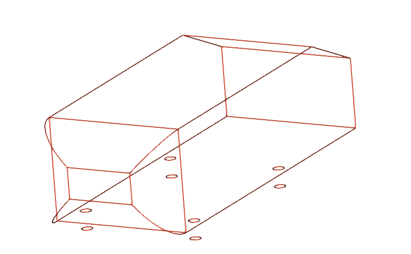
The dimensions of the Ahmed body are shown in Figure 1. The assumed air flow velocity is 60 m/s.
For a closer look at the meshing tutorial, please check out our help page.
Mesh Generation
Let us take a closer look at mesh generation and present the generation of meshes using Cartesian and tetrahedral meshing workflows in CF-MESH+. Most attention is paid to provide you with some guidelines how to consistently generate meshes for low-Re simulations of boundary layers.
One of the utmost important requirements when generating a mesh with very thin boundary layers is to resolve the geometry. In addition, variation of surface area vectors shall be slow on face-by-face basis. For geometries with sharp features, it is important to resolve those features before attempting to generate layers there. The Ahmed body has some sharp edges defined as feature edges, shown in the figure below. The feature edges are constraints that shall be preserved when generating a mesh. A good rule of the thumb is to avoid feature edge with acute angles, they are better replaced by blends when creating your geometry. If possible, it is best to avoid having features if possible, because in a world outside simulations, sharp edges do not exist.
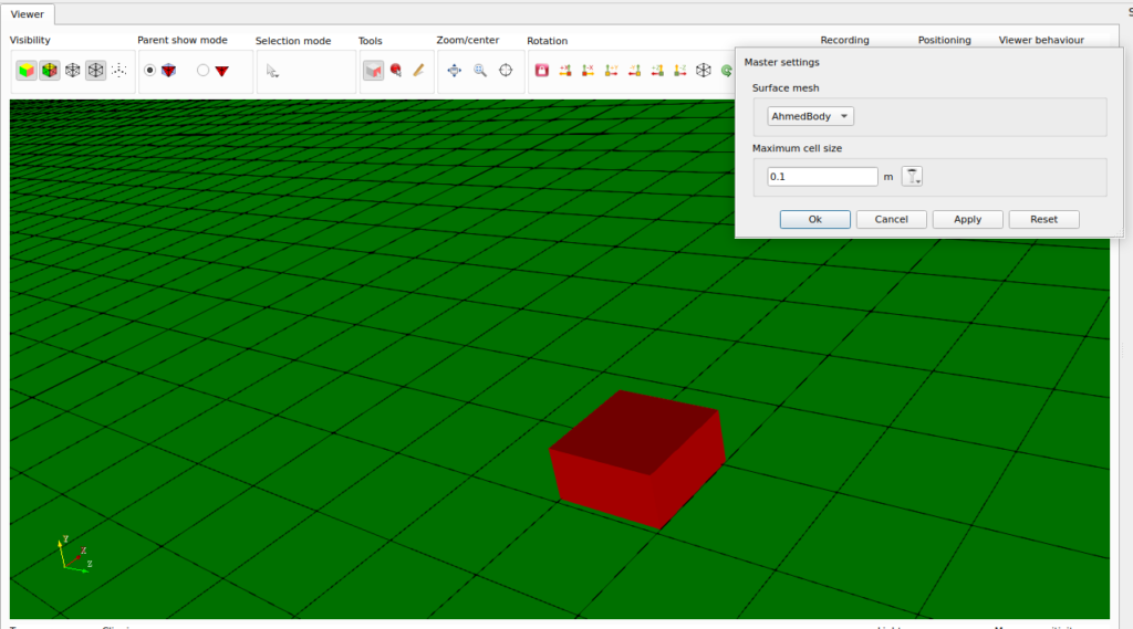
For the Cartesian mesh, the maximum cell size is set to 0.1 m.
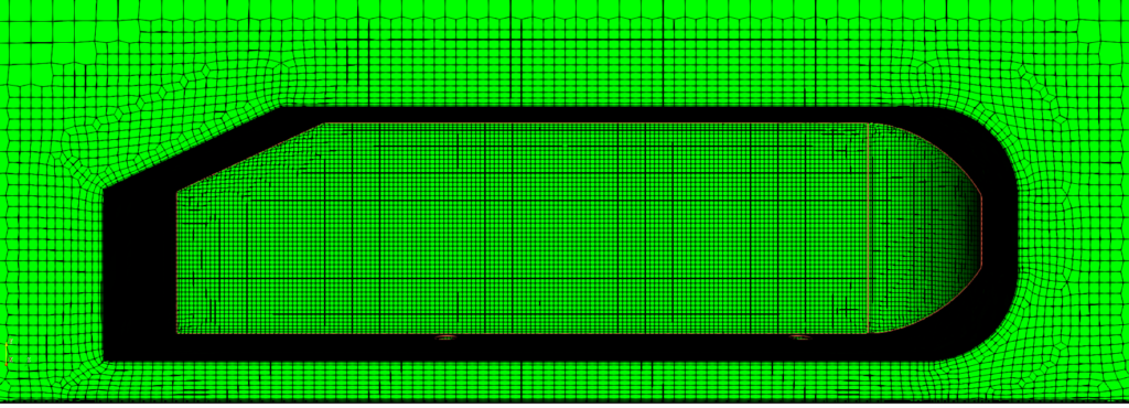
The mesh needs to be further refined near the Ahmed body to to be able to resolve the flow accurately. The mesh was also refined away from the body to avoid rapid transition of cells size in the region where the flow variation in rapid. It is always beneficial to keep the cell size uniform in regions of interest because it results in best possible quality of the resulting cells. It is especially beneficial to keep the cell size uniform near the feature edges to avoid rapid transition of cell size there, and avoid convergence problems.
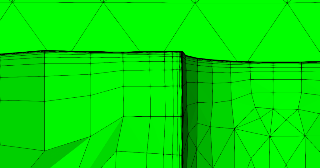
For the low-Re modelling the Y+ has to be smaller than one in the first layer cell at wall boundaries. Therefore, the first layer thickness was set to 6×10⁻⁶ m by using online Y+ calculator from CFD-online. The parameters for generating boundary layers are crucial because of rapid variation of flow variables compared to the rest of the volume. For low-Re layer modelling a good rule of the thumb it to use the total number of layer in the range between 15 to 25 layers. In this case, 15 layers were specified at walls. Out of the 15 layers 10 were specified as outer layers. This leaves 5 layers in the inner part of the layer whose first thickness and a thickness ratio of 1.1 are tightly controlled. In the outer part of the layer, the thickness ratio is calculated such that the smoothest possible transition between the inner layer and the outer layer is achieved. It is a good practice to specify more outer layers than inner layers, because the viscous part of the layer is very thin compared to the rest of the layer anyway, and this allows the mesher to gradually increase the cell size from the interior towards the rest of the mesh to achieve smooth transition of cell size outside the boundary layer. In general, it is advised to specify up to one third of the expected layer thickness as the inner part and leave the outer part for the mesher to resolve.
In addition, when generating thin boundary layers, it is also important to pay attention to the quality of the surface resolution to achieve high quality results. The most important details are:
- Avoid using unnecessary feature edges – these constraints are not necessary and result in lower mesh quality.
- Avoid having extremely sharp feature edges in the geometry – thin boundary layers require slow variation of normal from one boundary face to the other. Rapid variation of face normal vectors reduced mesh quality, and it is best resolved by creating blends in the geometry and refining the mesh locally.
- Avoid transition of cell size of sharp feature edges – it is also better to replace such edges with blends.
If the settings are done poorly, the mesher may struggle to generate a high-quality layer mesh, and it starts the fallback procedure, consisting of:
- Triangulation of base face – to resolve quality problems when the boundary faces are not flat.
- Merging of layers into a single layer – this indicates rapid normal variation of the layer.
- Collapse the layer locally – this is the last resort and most often occurs when the mesh is too coarse.

For the tetrahedral mesh, we aimed to have a similar number of cells, around 2.7 million. Since Cartesian cells are larger than tetrahedral cells, the maximum cell size in the tetrahedral case is set to 0.25 m. For the boundary layer, we used the same settings as for the Cartesian mesh.
For comparison, the Cartesian generated mesh has 8.14 million faces and 2.79 million points, while the tetrahedral mesh has 5.88 million faces and 0.82 million points.
CFD simulations
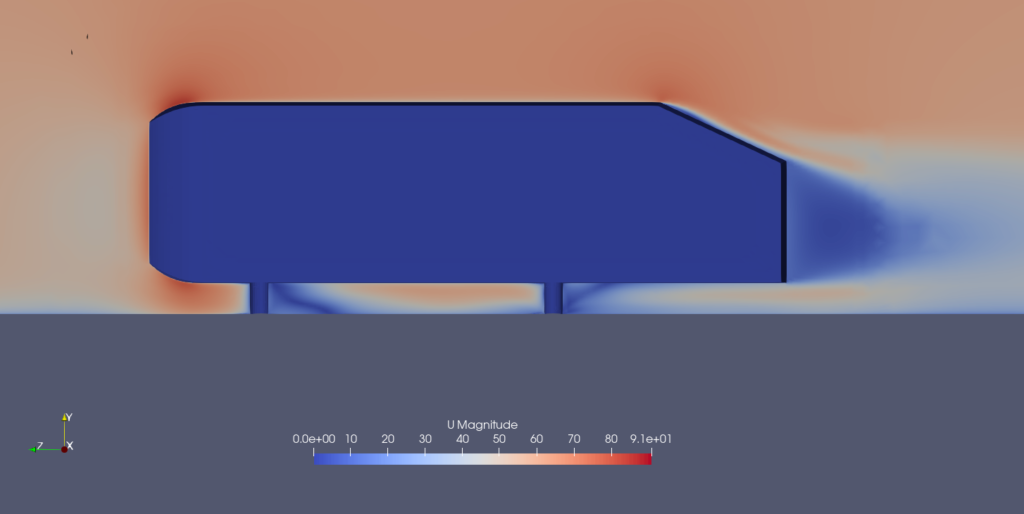
Both meshes were used for solving the flow at 60 m/s, by using the simpleFoam solver from OpenFoam-v2206.
Turbulence is modelled using the kOmegaSST model, and the kinematic viscosity of air is set to 1.5×10⁻⁵.
Discretisation schemes used for the simulations are:
| Gradient schemes | default cellMDLimited Gauss linear 1; grad(U) cellLimited Gauss linear 1; |
| Convection term schemes | default none; div(phi,U) bounded Gauss vanLeerV; div(phi,k) bounded Gauss limitedLinear 1.0; div(phi,omega) bounded Gauss limitedLinear 1.0; div((nuEff*dev2(T(grad(U))))) Gauss linear; |
| Laplacian schemes | default Gauss linear corrected; |
| Interpolation schemes | default linear; |
| Surface-normal gradient schemes | default corrected; |
| Wall distance calculation scheme | method meshWave; |
Boundary conditions:
| Patch | k | nut | omega | p | U |
| AhmedBody | Fixed value 0.0 | NutLowReWallFunction 0.0 | Wall-function | Zero gradient | No slip wall |
| Bounding box | Fixed Value 0.0 | NutLowReWallFunction0.0 | Wall-function | Zero gradient | No slip wall |
| Inlet | Fixed Value 4.86 | Calculated 0 | Fixed Value 22.05 | Zero gradient | Fixed value (0 0 -60) |
| Outlet | Inlet Outlet 4.86 | Calculated 0 | Inlet-outlet B.C. | Fixed value 0 | Inlet outlet (0 0 -60) |
| Road | Fixed Value 0.0 | NutLowReWallFunction0.0 | Wall-function | Zero gradient | No slip wall |
| Symmetry planes | Symmetry plane | Symmetry plane | Symmetry plane | Symmetry plane | Symmetry plane |
Simulation of both meshes shows similar drag and lift coefficients, the drag coefficient for the cartesian mesh simulation is 0.2388, and the lift coefficient is 0.00029, while for the tetrahedral mesh solution the drag coefficient is 0.2390, and the lift coefficient is 0.00030. Calculations of Y+ values at all wall boundaries show that the Y+ is smaller than one at all wall faces in the mesh.
In general, the solutions on tetrahedral meshes are expected to contain an order of magnitude higher discretisation errors in the solution for the same number of cells compared to the mesh consisting of hexahedral cells. However, by looking at the flow, it can be noticed that in most parts of the domain the flow is almost uniform, and any mesh can resolve it accurately, and significant variations are present in the boundary layer in the direction normal to the wall, which is resolved with high-quality boundary layers. Hence, the differences in the results obtained are not as large as it may be expected. Therefore, paying attention to generating a high-quality boundary layer mesh helps in getting most out of your CFD modelling efforts.
We hope that you have found this post useful and that it has made you curious to try out our latest CF-MESH+, designed to alleviate the pain of meshing. You can also subscribe to our newsletter to stay informed on our newest developments.
- How to install a trial version of CF-MESH+
- Our best meshing practices for high-quality CFD simulations
- Is it always the mesh? Part 7: Volume Ratio – the Secret Killer Nobody Talks About
- Automatic Acute Edge Detection and Fillet Creation Algorithm
- Join us at the upcoming webinar “Next-Gen Meshing Technology at IANUS” with CF-MESH+
")
