Introduction: The Katabatic Challenge
Simulating wind over complex terrain is a well-established area of environmental CFD, but the Croatian wind Bura presents unique numerical challenges. Unlike standard atmospheric boundary layers driven by freestream gradients, the Bura is a severe katabatic wind – a dense, cold pool of air that spills over the Velebit mountain range and plummets toward the Adriatic Sea. It is highly compressible, density-driven, and interacts violently with extreme topography.
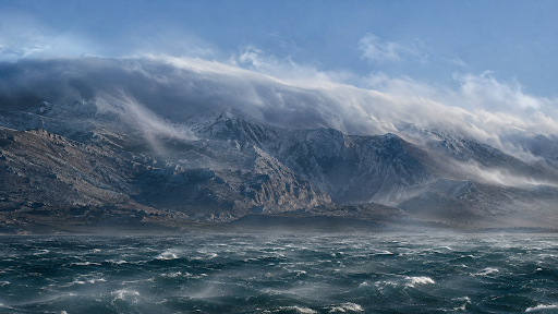
Standard FVM atmospheric assumptions are often insufficient in this regime. In this article, a stable, production-ready workflow for simulating the Bura over the Paklenica canyons is presented, starting from raw geolocation data and concluding with a stable OpenFOAM computation.
Step 1: Sourcing the Terrain Data
Obtaining high-quality topographical data has been greatly simplified by modern GIS tools.
Standard geolocation services and GIS applications (such as QGIS with the OpenTopography plugin, or web-based STL exporters like Terrain2STL, Map2Model, etc.) can be utilized to capture the exact coordinates of the Velebit mountain range. The region of interest is selected, and the raw 3D surface is exported directly as an STL file. This single STL file serves as the sole geometric input required to initiate the meshing process.
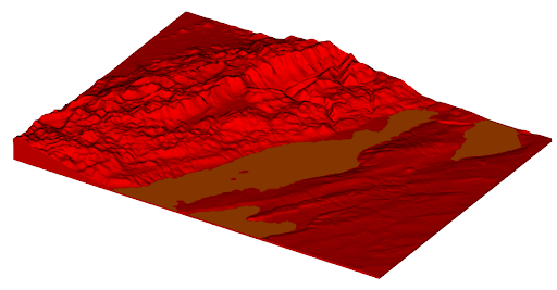
Figure 1 Terrain exported from the web
Step 2: The CF-MESH+ Workflow
Generating a high-quality computational mesh over complex, jagged mountainous terrain is frequently considered the primary bottleneck in environmental CFD. However, this process is significantly simplified within CF-MESH+.
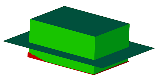
Figure 2 Geometry of computational domain
Manual stitching of surfaces or the construction of complex block topologies is not required. The workflow is reduced to two primary steps:
- Defining the Bounding Box: After the terrain STL is imported, a primitive bounding box is created around the terrain to establish the outer limits of the computational domain (defining the lateral boundaries, and the sea). A horizontal plane is inserted at 4000m representing the top boundary. By doing so it is easy to replace the top boundary and generate a new plane at a different height.
- Automated Volume Meshing: Upon intersection of the bounding box and the terrain STL, the fluid volume is automatically identified by the software. Refinement zones are created near the boundary and boundary layers are generated over all wall patches, see Figure 3 Refinement settings. inletOutletPatches settings were used to ensure that boundary layers exit the domain at all inlets and outlets, as shown in Figure 4 Boundary layer settings.
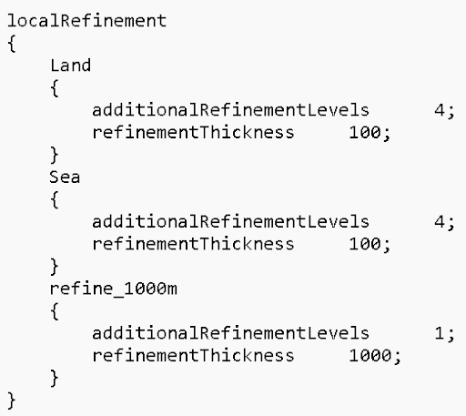
Figure 3 Refinement settings
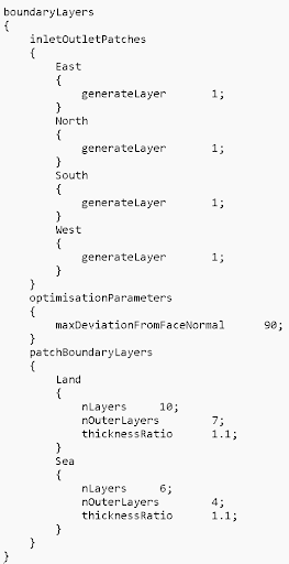
Figure 4 Boundary layer settings
By applying local refinement zones near the Paklenica canyons and elsewhere near the ground all geometric features can be resolved. Refinement inside the volume near the ground is achieved by using the refinementThickness option, Figure 3 Refinement settings. Ten boundary layers are generated over the land and six layers are generated over the sea patch, Figure 4 Boundary layer settings.
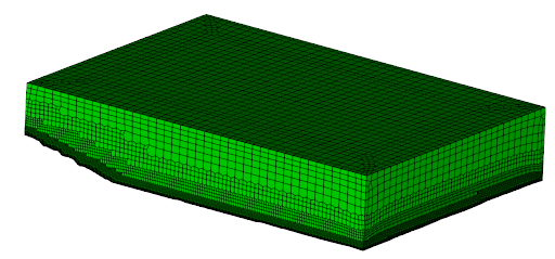
Figure 5 Volume mesh
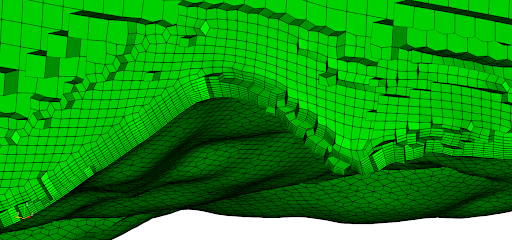
Figure 6 Boundary layer and the mesh near the ground
Simulation Setup and Boundary Conditions
When dealing with a domain spanning 4000 vertical meters, the hydrostatic background pressure (ρg·h) completely dominates the dynamic pressure variations.
Attempting to solve for absolute thermodynamic pressure directly forces the boundary conditions to mathematically balance a massive gravitational vector, which frequently causes an accumulation of mass. This problem is solved by utilizing OpenFOAM’s standard buoyantPimpleFoam solver, which natively solves for the modified pressure field (p_rgh = p – ρg·h). This approach elegantly isolates the dynamic katabatic wakes from the background barometric weight. Turbulence was modelled using the standard k-epsilon turbulence model with standard coefficients.
The specification of open boundaries was the biggest challenge because inlets and outlets require special treatment to avoid violating hydrostatic equilibrium. Boundary conditions were specified as:
- North and East boundaries serve as the inflow of the fluid. In a private communication with a colleague specializing in Wind Engineering, he mentioned that such extreme conditions generate a quite uniform velocity profile. Hence, we specified velocity as a uniform value of (8, 8, 0) m/s and set it to vary linearly from zero at the ground to the specified value in the first 200 meters near the ground. Turbulence properties were set using the atmBoundaryLayerInletK and atmBoundaryLayerInletEps. The temperature profile assumed stable atmospheric stratification with a temperature gradient of 6.5 C/km. fixedFluxPressure boundary condition is used for the p_rgh field.
- South and West boundaries serve as the outflow of the fluid. A zero gradient boundary condition was applied to turbulence fields and temperature. In order to account for the large differences in pressure, the prghPressure condition was used for the pressure, and the value was specified using the formula for the hydrostatic pressure. This proved to be a crucial step because it stabilizes the pressure equation and avoids pressure drifts to extreme values. The pressureInletOutletVelocity condition was used for the velocity field to avoid reflections of pressure waves back to the computational domain.
- The Land patch is modelled as an adiabatic boundary, allowing the downslope Bura to undergo natural dry adiabatic warming as it descends. Turbulence properties and velocity were modelled using the atmospheric boundary layer wall function with z0 equal to 0.5 m.
- The Sea patch is modelled as a fixed temperature boundary at 288 K. For turbulence properties and velocity, an atmospheric wall function with z0 equal to 0.001 m is applied.
- The Sky patch is modelled as an inletOutlet patch for the velocity field and temperature. prghPressure boundary condition is applied on the pressure and the static pressure is assigned according to the hydrostatic pressure formula. Zero gradient condition is used for turbulence fields.
Initial conditions inside the domain are set using the setExprFields utility to set the pressure and temperature. This is primarily needed to stabilize the simulation in the first couple of time steps and avoid problems with mass conservation.
Laplacian terms are modelled using the Gauss linear limited 0.5 scheme. Convection terms in the momentum equation are approximated with the Gauss limitedLinearV 1.0 scheme. Gauss vanLeer was used for the energy equation and Gauss linearUpwind cellMDLimited Gauss linear 1.0 for turbulence equations. Temporal discretisation is achieved by using the Euler scheme with variable time step with max Courant number of 0.5.
Results
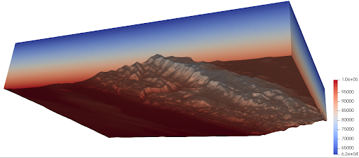
Figure 7 Pressure field
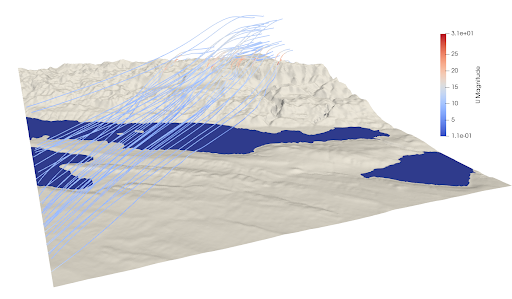
Figure 8 Wind blowing down the ridge
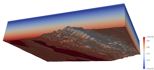
Figure 9 Temperature field
The preceding figures illustrate the spatial distributions of pressure, temperature, and velocity. Seeded within the 200-meter inversion layer at the inlet, the streamlines effectively trace the descent of the dense cold pool as it cascades down the topography and begins to warm upon reaching the sea. While localized gusting is a physical hallmark of this flow, the domain-wide maximum velocity plotted in Figure 10 primarily demonstrates the successful bounding and stabilization of the initial numerical transient. As the current simulation was executed for thirty-eight seconds, the computational runtime must be extended in future studies. Longer physical simulation times, coupled with localized probe sampling, will be required to determine if this framework can accurately capture rapid micro-gusts (30–60 second intervals) alongside the broader, quasi-periodic Bura pulsations that typically cycle every 3 to 11 minutes.
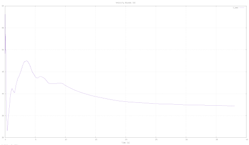
Figure 10 Maximum observed velocity with time
Conclusions and Future Work
This post demonstrates a simulation of severe, compressible katabatic Bura wind. These kinds of flows can be stably and efficiently modeled, starting from a simple STL download of the location of interest. Meshing in CF-MESH+ is simple, takes a few minutes, and does not require a high-quality surface mesh to generate a high-quality volume mesh with smooth boundary layers needed to capture shear stresses at the ground and sea. The next evolutionary step involves calibrating the aerodynamic roughness (z0) and thermal fluxes of this numerical environment against physical measurement masts deployed by Wind Engineering teams along the coast. Additionally, extended physical simulation times and the deployment of localized numerical probes will be required to definitively prove whether this computational framework can successfully reproduce the characteristic high-frequency micro-gusts and overarching quasi-periodic pulsations of the Bura flow.