Quite often I hear warnings about “unacceptable” aspect ratios, claims that they ruin simulations, and debate on when stretching is acceptable versus dangerous. The point of this series of posts is to demystify popular myths, help you understand what is happening physically and mathematically inside your Finite Volume CFD code, and guide you on how to interpret mesh quality metrics and the obtained results. In this post, we tackle the influence of aspect ratio, and how extreme stretching – even on pristine meshes – can sometimes break your solver.
Aspect Ratio – Definition
In mesh generation and CFD literature, aspect ratio is often defined by a ratio of bounding dimensions (e.g., Lmax / Lmin). While intuitive on paper, this definition has a severe flaw in automated mesh generation: when an element degenerates or features a zero-area face, it leads to a division by zero and/or unbounded numbers.
To ensure robustness, we define the aspect ratio (Ar) of a cell as the quotient of the area magnitude of its smallest face divided by the magnitude of its largest face:
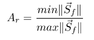
This robust metric is bounded: 0 < Ar ≤ 1. Perfectly isotropic cells have Ar = 1, while highly stretched cells have Ar → 0. By using the largest face area as the denominator, the metric is always stable and avoids singular divisions.
Motivation: The Supersonic Failure Scenario
To understand why small aspect ratio affects the solver, let’s explore an example that perfectly illustrates the conflict between geometric perfection and physical stability.
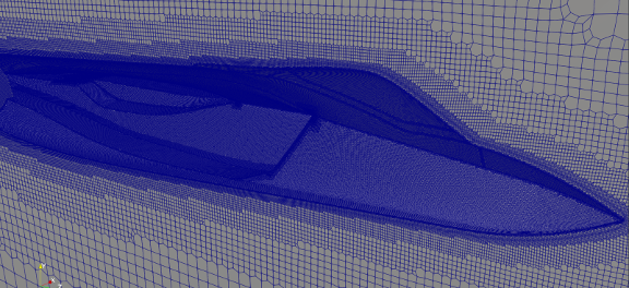
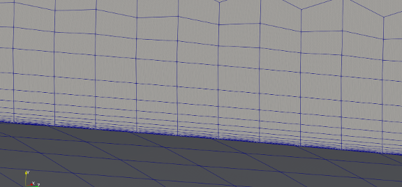
I wanted to check if it is possible to do a low-Re simulation of a supersonic flow on an aircraft. We know that CF-MESH+ is capable of generating high-quality boundary layers, and I wanted to push it to the extreme and generate very thin layers to perform a low-Reynolds simulation of a supersonic flow over an F35 aircraft using y+ ≈ 1. I soon noticed that while the boundary layer mesh looks aesthetically perfect – see Figure1 and Figure 2 zoomed view and the large external fuselage view – the simulation itself did not converge to a physically meaningful result.
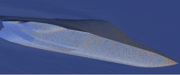
The pressure field in the boundary layer did not converge to a physically meaningful field; instead, unphysical odd-even fluctuations, or checker-boarding, developed specifically where the highly stretched cells were located on the fuselage surface, see Figure 3.
What is causing this problem?
The core of the issue is not the mesh quality, but the interaction between the discretisation practice and the physical flow dynamics, resulting in a matrix with negligible coefficients at small faces. The oscillations occur in the boundary layer at the boundary where the diffusion is dominant, hence, we will limit the analysis to the Laplacian term used for modelling the viscous forces.
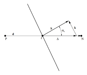
Let us start by discussing the Finite Volume discretisation practice of a standard a Laplacian term for a scalar quantity φ. On a general non-orthogonal mesh, shown in Figure 4, the approximation of the Laplacian term can be written:
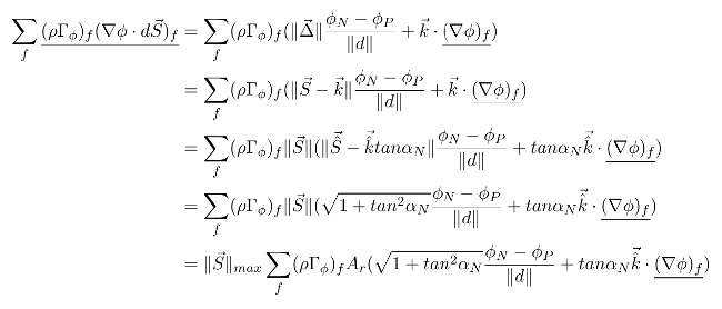
Where Ar represents the aspect ratio of a face measured by the area of the largest face in the cell. In addition, it also noticeable that non-orthogonality angle influences the accuracy of the approximation, too, as discussed in one of previous posts about non-orthogonality. This generic form only shows that small aspect ratio reduces the weight of a neighbour cell in the matrix and nothing more can be said at this point.
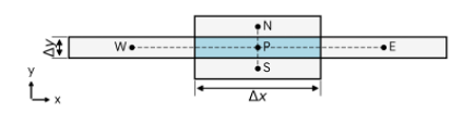
In practice, anisotropic cells are used in boundary layers and shear layers inside the domain. In most cases, anisotropic cells are of prismatic type such that their height can be small compared to the area of the base. In order to simplify the analysis, let us analyse an orthogonal stretched quad cell in 2D space, because the same analysis also applies to 3D prisms.
Let us now calculate the ratio of the fluxes at the west and the north faces. It can be written as:

Knowing that the mesh is orthogonal, and that the density and viscosity do not change much locally, the equation can be simplified to:
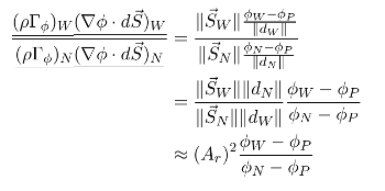
This equation shows that the coefficient at the western faces quickly becomes small compared to the coefficient at the north face. This results in a decoupled system, prone to unphysical oscillations because the influence of the western and eastern faces is negligible in the matrix.
Therefore, even though the mesh in the F35 example was geometrically pristine, high quality, and generated perfectly by CF-MESH+, the simulation failed because the linear system characteristics created by the extreme stretching simply exceeded the mathematical stability limits of the standard segregated iterative solver.
Key Takeaways
- A Numerically Stable Metric: Defining aspect ratio as min |Sf| / max |Sf| avoids singular divisions, bounding Ar within the interval (0, 1].
- Matrix Decoupling: Small aspect ratios cause matrix coefficients along the stretched faces to collapse quadratically with the reduction of the aspect ratio resulting in a decoupled system prone to checkerboarding and spurious oscillations.
- Decoupling is not always failure: When physical fluxes are 1D normal to the wall, the decoupling aligns with the physics and the extremely small aspect ratios do not cause harm because the contribution of small face is negligible anyway.
- Catastrophic failures may occur when multi-dimensional physics occurs over the small faces and it cannot influence the value in the cell because small Ar makes it negligible. This gets manifested as unphysical oscillations.
The goal of this post was to analyse the influence of aspect ratio on the stability of the Laplacian term. I hope that you find this analysis useful for your CFD work, and I hope this will motivate you to try CF-MESH+. The aspect ratio is one the metrics showing that it is not always the mesh responsible for problems in getting accurate results. Even though a double precision solver was used, it still was not enough for such an extreme case.
You can stay tuned for the analysis of the convection term, by signing up for our newsletter.