Introduction
The process of importing CAD files has become simpler, more efficient, and packed with enhanced functionalities in the latest update to CF-MESH+. Users can now seamlessly import .step, .iges, and .brep files via the command line using the new CADToFMS utility or through the familiar GUI “Import CAD” tool. Say goodbye to tedious setup processes for complex geometries – our improved import for .step files organizes subassemblies into face subsets and named parts into patches, streamlining your case setup. Additionally, you can effortlessly import multiple CAD files at once, which are then merged into a single surface mesh. Plus, our new enhancement automatically collects face subsets based on CAD curvature values, paving the way for automatic refinement and easier case configuration. The new feature will be explained using an example of a Jet case setup, where we will also explain how to achieve the desired y+ using our boundary layer settings for this type of case.
CAD import
To demonstrate the functionality of our new utility, let’s walk through the process using the “Jet_CAD.step” geometry file, which was downloaded from GrabCAD and saved as Jet_CAD.step with the assembly tree shown below.
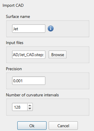
In the new utility, you can specify the following parameters:
- “Surface name”: This represents the name of the output surface mesh.
- “Input files”: Here, you can select multiple .iges, .brep, or .step files.
- “Precision”: This parameter represents the relative linear deflection or the maximum allowable deviation between the meshed representation and the original faces, curves, or edges of the CAD model. Absolute linear deflection is calculated as the smallest dimension of the bounding box, multiplied by the user-defined precision value. The default precision value is 0.001.
- “Number of curvature intervals”: This parameter represents the number of intervals in which curvature results will be distributed and written into dedicated subsets.
The “Jet_CAD.step” file comprises an assembly tree-structured as follows:
Jet (Main assembly)
– MainWings
– Engines
– TailWings
– Fuselage
After importing the file, the surface mesh within the project tree appears as depicted in the following image:
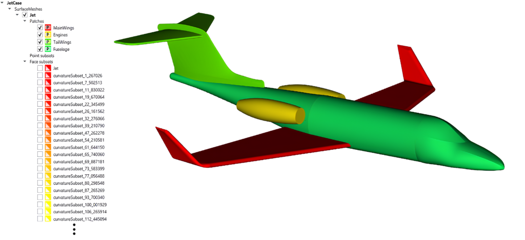
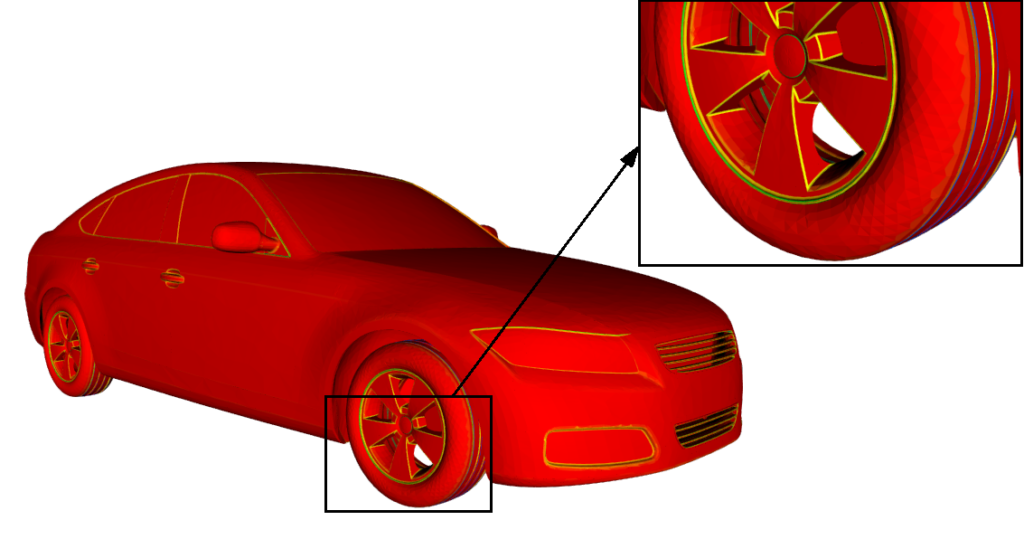
For the provided CAD geometry, we utilized the default value for the number of curvature intervals (128), resulting in 79 curvature face subsets due to the distribution of these curvature values (ranging from 1 to 919). These curvature subsets are labeled as ‘curvatureSubset_IntegerPart_FractionalPart’, where the Integer and Fractional parts represent the integer and fractional portions of the curvature values.
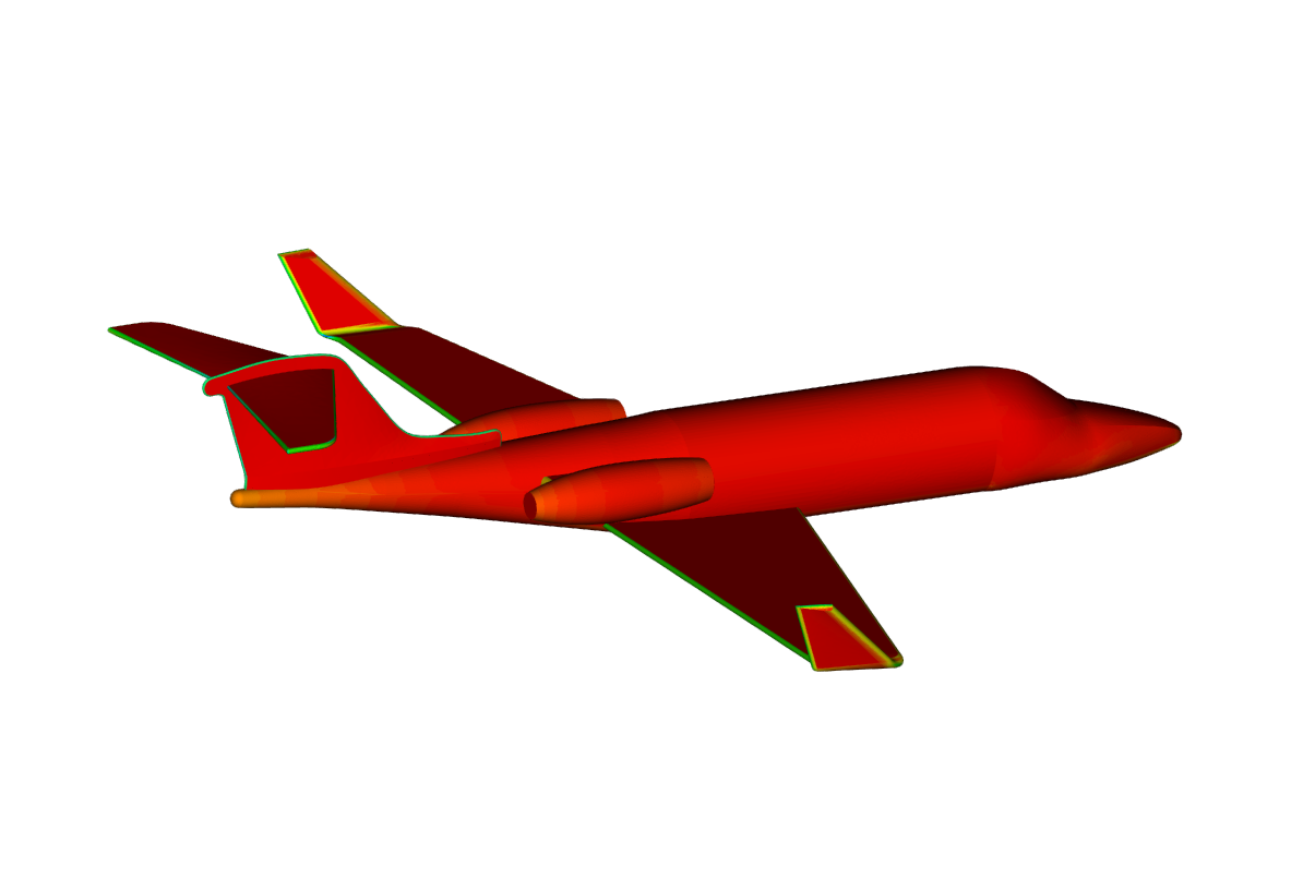
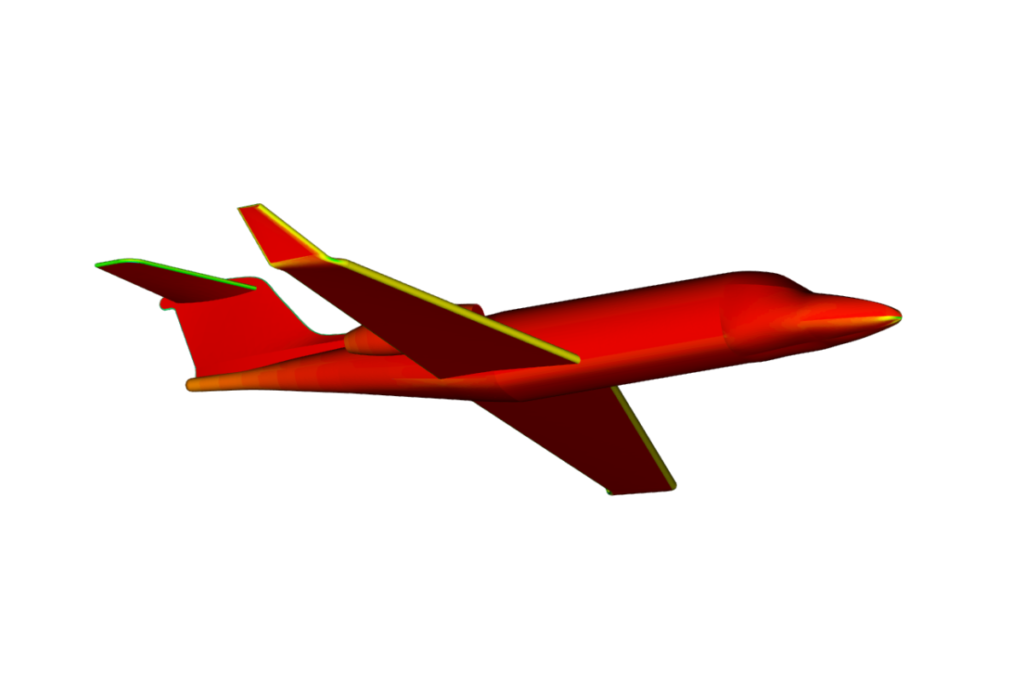
The following images illustrate how the curvature values are represented in the resulting surface mesh.
If you plan to utilize automatic curvature refinement based on CAD curvature information, it is advisable to refrain from renaming or modifying curvature subsets. Once you employ automatic curvature refinement, if the curvature subsets exist within the mesh, automatic curvature refinement will utilize the data provided by those subsets. However, if they do not exist, the mesher will calculate the curvature values in the same manner as in previous versions.
It’s important to note that the “precision” value limits the maximum curvature value in a given geometry. Therefore, if you aim to capture subsets with higher curvature values, you will need to lower the precision value accordingly.
To illustrate how curvature subsets appear in a different example, here’s an example of a
DriveAer geometry (obtained from TU Münich). This example will also be updated in the future to feature a much cleaner and simpler setup, utilizing curvature automatic refinement and the new “Import CAD” curvature subsets.
We encourage users to experiment with various precision values to understand how they affect the output surface. Keep in mind that when using very small precision values, it may take some time for the algorithm to achieve the desired high-precision surface.
Case setup
After importing the geometry, it is essential to add a bounding box of the correct size to accurately capture the flow around the Jet aircraft. This can be achieved by right-clicking on primitives in the project tree, and navigating to Primitives -> Add -> Box/bounding box.
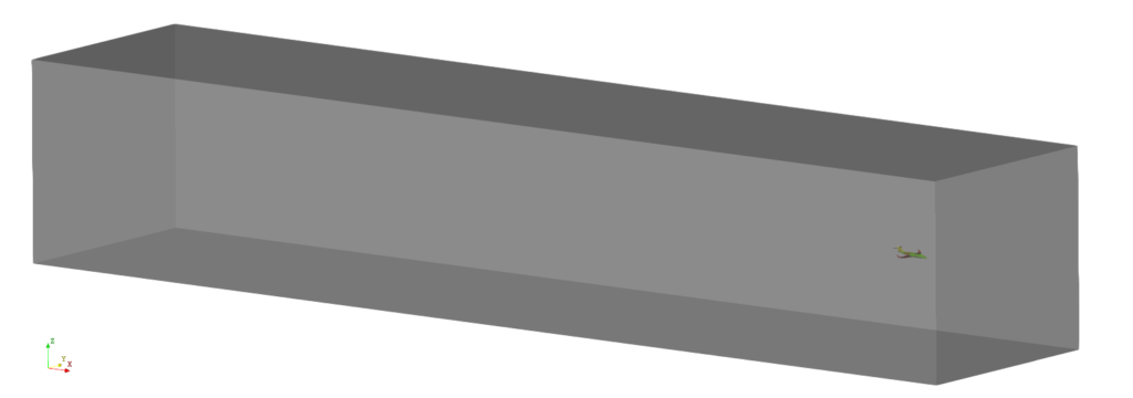
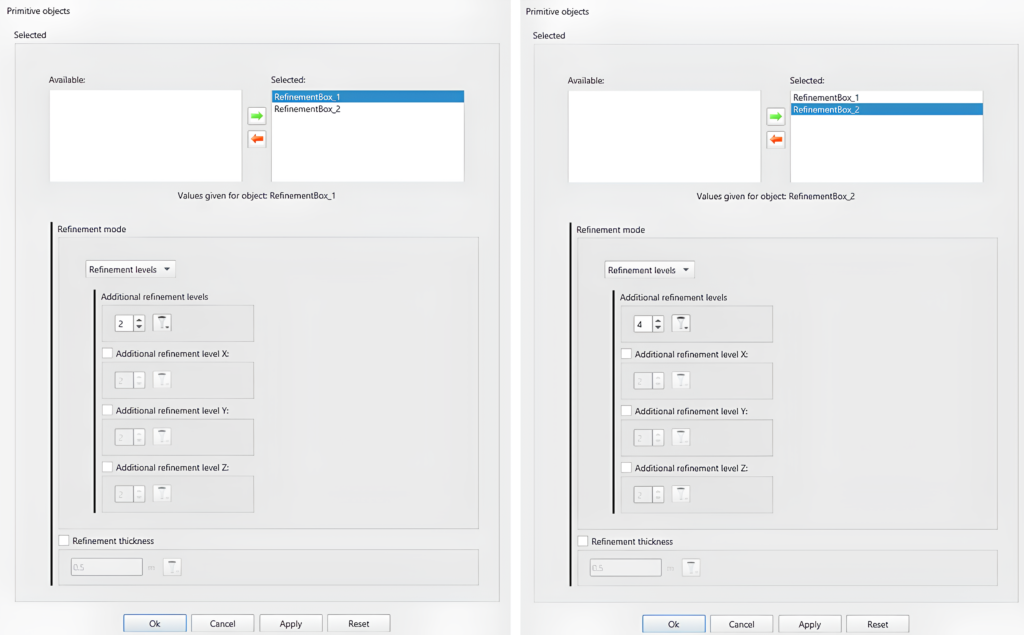
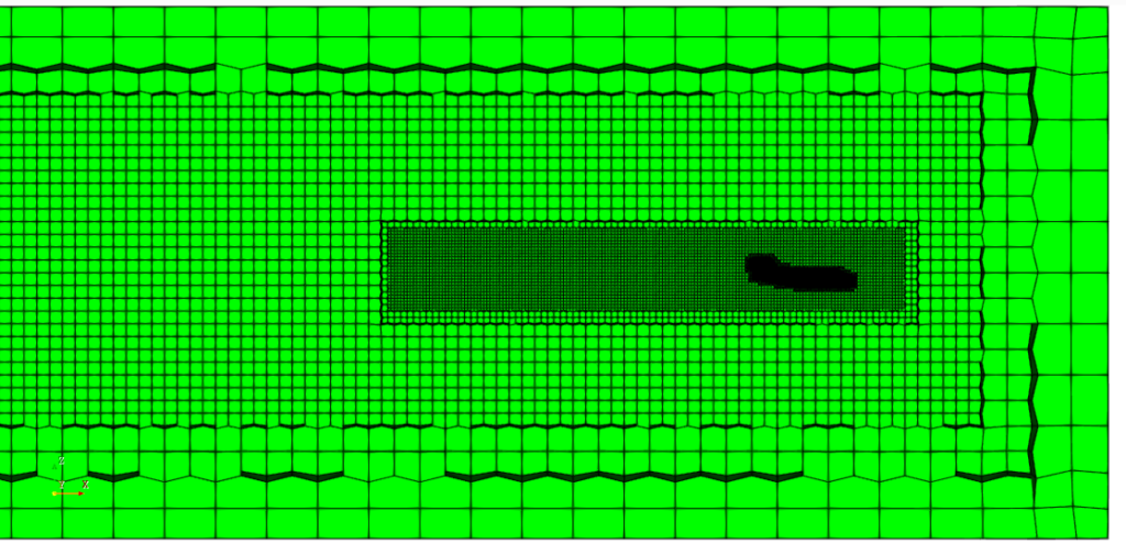
Additionally, two smaller primitives will be added for refinement purposes, which will be visible later in the case setup and in the final volume mesh.
Now, setting up a case is a breeze, requiring just three simple steps:
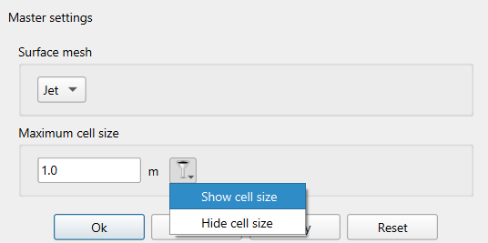
1) Master settings
Here, we select the maximum cell size, which for our domain size will be set to 1m as an experimental value. You can use the “show cell size” tool, as shown in the picture below, to determine your desired maximum cell size. (Please note that the .step file being utilized represents a scaled model of the Jet, which is downsized by a factor of 10 compared to the actual dimensions. The scaled model measures 1.9×1.8×0.4 m.)
2) Refinement sources
In this step, we implement three types of refinement. Firstly, we refine the face subset representing the entire jet’s main assembly to achieve cell uniformity across the surface.
Secondly, we refine the primitive objects previously created to capture the flow gradients around and behind the jet
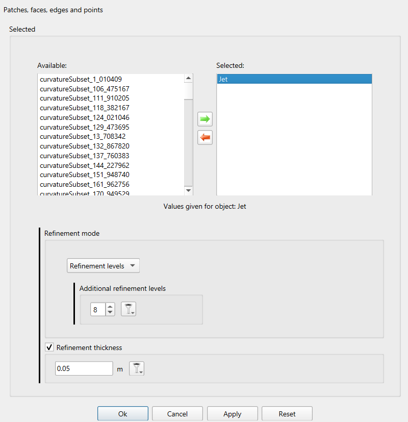
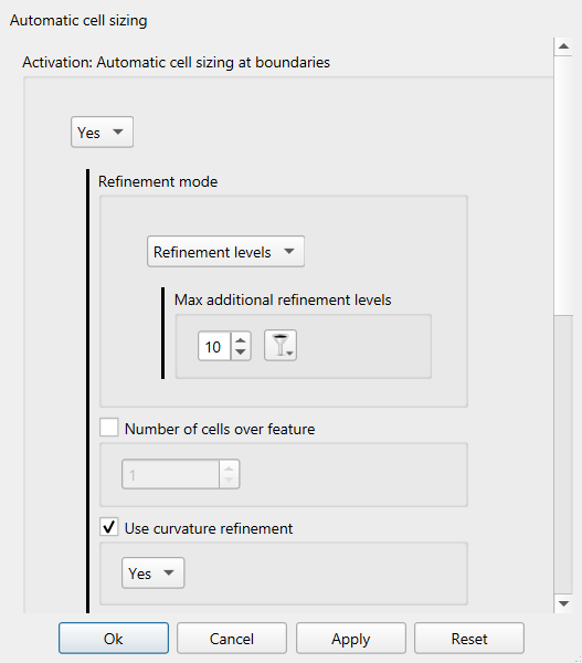
Lastly, we enable automatic refinement, specifying the number of additional refinement levels. Once again, you can utilize the “show cell size” tool to determine the required number of additional refinements. Additionally, we enable “Use curvature refinement,” which utilizes “curvatureSubsets” data if they exist in the surface mesh, as explained earlier.
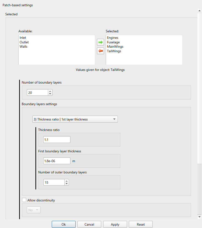
3) Boundary layers
We define boundary layers on all patches representing the surface of the Jet.
As stated in the introduction, we will explain the proper utilization of our boundary layer settings for this specific case type. Given that the discretization error diminishes rapidly as one moves away from the wall, it becomes crucial to prioritize smooth thickness variation within the inner part of the layer. This approach ensures accurate resolution of shear stress, which is precisely achieved through the application of specified settings. If you want to delve deeper into boundary layer theory, feel free to explore our latest post, which provides a comprehensive explanation of the topic.: Is it Always the Mesh? Part 5: Boundary Layer Meshing.
We utilized the 3) Thickness ratio | 1st layer thickness option, as depicted in the image above. With this option, the inner portion of the boundary layer is controlled by the specified thickness ratio (We have set a total of 20 layers, dividing them into inner and outer layers. With 15 outer layers configured, the remaining 5 layers constitute the inner layers). Moreover, in the outer section of the layer, the implemented algorithm ensures the optimal outer thickness ratio, facilitating a smooth transition between the inner part of the layer and the internal mesh. To attain the desired y+ value, it’s essential to calculate the desired first layer thickness. If you’re unsure how to perform this calculation, we recommend utilizing an online wall distance estimation calculator.
Mesh overview
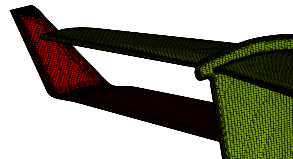
The final mesh comprises 13684457 cells, including 20 boundary layers surrounding the Jet. Additionally, refinements are incorporated to effectively capture flow gradients in the wake behind and around the jet, ensuring a comprehensive representation of the flow dynamics.
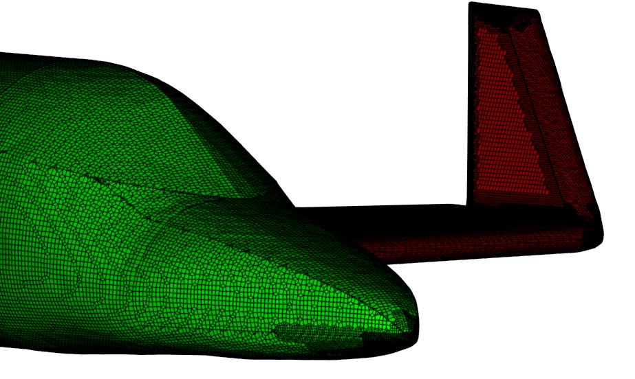
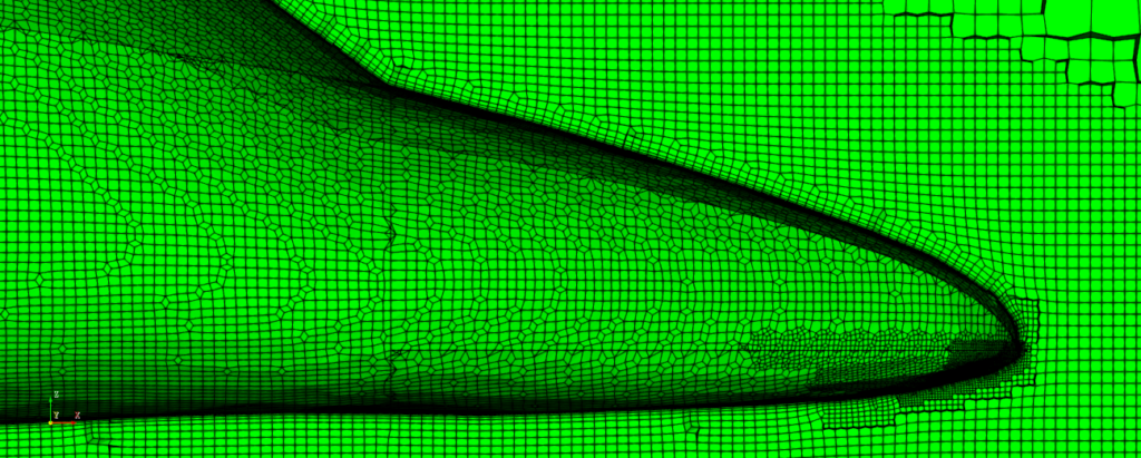
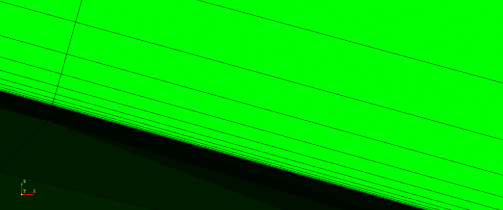
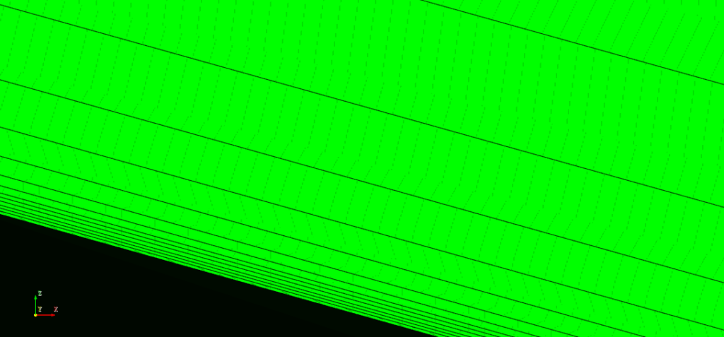
As depicted in the following images showcasing the patches of the volume mesh, we’ve successfully translated the surface mesh into a comprehensive volume mesh representation, accurately capturing the intricacies of the Jet’s surface. The next two pictures illustrate the surface with the volume mesh edges, providing insight into how the given curvature subsets, in combination with automatic curvature refinement, operate to enhance the mesh quality.
The subsequent picture displays the volume mesh cut through the middle of the Jet, highlighting the primitive refinements.
The following three pictures will demonstrate the functionality of our boundary layer algorithm, focusing on the outer and inner layers discussed previously. These images also display the volume mesh cut through the middle of the Jet. In the first two pictures, you can observe how the outer part of the layer smoothly transitions to the internal mesh.
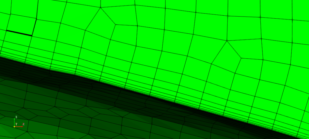
With the first layer thickness set at 1.8e-6 m, extensive zooming is necessary to discern the inner layer which is uniform across the entire Jet surface. In the subsequent picture, only the outer part of the layer is visible, while the second image reveals the inner part of the layer, which is too small to be observed in the first image.
I hope that you have found this post useful and that it has made you curious to try out CF-MESH+ and its CAD to FMS feature. You can also subscribe to our newsletter to stay informed on our newest developments.
- How to install a trial version of CF-MESH+
- Our best meshing practices for high-quality CFD simulations
- Is it always the mesh? Part 7: Volume Ratio – the Secret Killer Nobody Talks About
- Automatic Acute Edge Detection and Fillet Creation Algorithm
- Join us at the upcoming webinar “Next-Gen Meshing Technology at IANUS” with CF-MESH+
")
